I started this project with a simple question. How can a system identify a song from just a few seconds of audio?
At first, this felt like one of those problems that must rely on heavy machine learning or large neural networks. After reading Shazam’s original paper and exploring projects like Dejavu, I realized the core idea is much more elegant. Audio fingerprinting is mostly about signal processing and efficient database lookups.
This post walks through how I built an end to end audio fingerprinting system in Python that can download music from YouTube, fingerprint tracks, store them efficiently, and identify songs from short audio clips.
You can check out the code on GitHub: sakkshm/spectra or try it out for yourself at: Spectra
Representing Music as Data
Digital audio is just a sequence of numbers. In a typical .wav file sampled at 44,100 Hz, each second of audio contains 44,100 samples per channel. A three minute song contains millions of samples.
Looking at raw samples directly is not very useful. Most of the information we care about in music lives in the frequency domain, not the time domain.
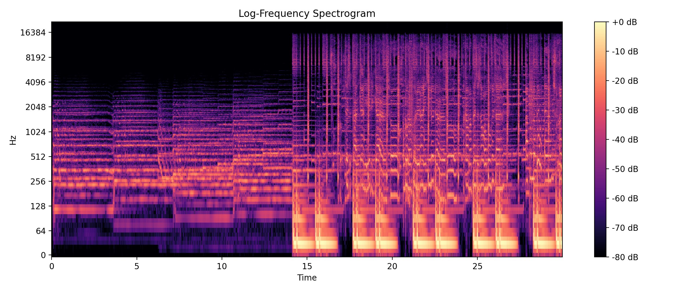
To extract that information, I apply a Short Time Fourier Transform(STFT). This splits the signal into small overlapping windows and computes the frequency spectrum for each window. The result is a spectrogram, a two dimensional representation with time on one axis, frequency on the other, and amplitude as intensity.
In Python, this step is handled using librosa:
y, sr = librosa.load(path, sr=22050, mono=True)
S = np.abs(librosa.stft(y, n_fft=4096))
S_db = librosa.amplitude_to_db(S, ref=np.max)
Each point in the spectrogram represents how strong a particular frequency is at a particular moment in time.
Why Peaks Matter
A spectrogram contains a lot of information. Most of it is not stable enough to use as an identifier. Small changes in volume, noise, or compression can distort many values.
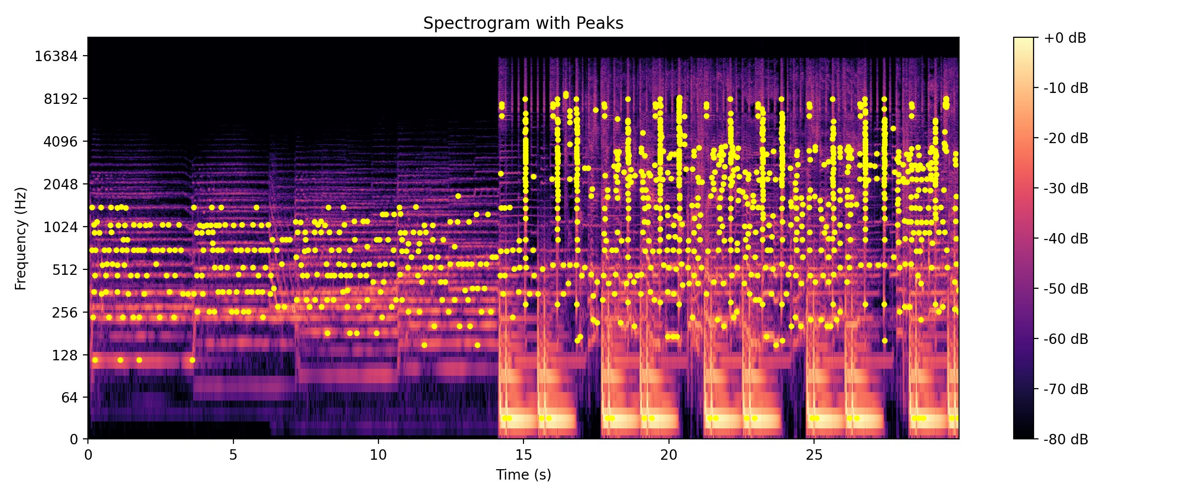
What tends to survive these distortions are local maximas. These are points in the spectrogram where a frequency has significantly higher energy than its neighbors. The idea is to detect these peaks and ignore everything else.
To do this, I use a two dimensional maximum filter over the spectrogram. For each time frequency point, I check whether it is the strongest value in a local neighborhood.
from scipy.ndimage import maximum_filter

neighborhood = maximum_filter(S_db, size=(15, 15))
peaks = (S_db == neighborhood) & (S_db > threshold)
Each detected peak can be represented as a tuple of time index and frequency index.
These peaks are surprisingly robust. Even if the song is recorded through speakers or compressed heavily, many of the same peaks still appear.
From Peaks to Fingerprints
A single peak is not very meaningful by itself. The real insight is to combine peaks into pairs (called constellations).
For each peak, I look ahead in time and pair it with other nearby peaks. Each pair forms a fingerprint that captures the relationship between two frequencies and their time difference.
A typical fingerprint encodes:
- Frequency of the anchor peak
- Frequency of the target peak
- Time difference between them
These values are concatenated and hashed using SHA 1. The hash becomes the fingerprint.
hash_input = f"{f1}|{f2}|{dt}".encode()
fingerprint = hashlib.sha1(hash_input).digest()[:10]
Using peak pairs increases entropy and dramatically reduces collisions between songs. Only the first 10 bytes of a SHA-1 hash are stored. This keeps storage compact while preserving enough uniqueness for reliable matching.
Each fingerprint is stored along with the song ID and the time offset of the anchor peak.
Database Design
The database is intentionally simple. There are two main tables.
Songs table
Stores metadata and an identifier.
CREATE TABLE songs (
    song_id SERIAL PRIMARY KEY,
    song_name VARCHAR(250),
    fingerprinted BOOLEAN DEFAULT FALSE
);
Fingerprints table
Stores binary hashes and timing information.
CREATE TABLE fingerprints (
    hash BYTEA NOT NULL,
    song_id INT NOT NULL,
    offset INT NOT NULL,
    UNIQUE (song_id, offset, hash)
);
The hash column is indexed. This is critical. During matching, the system performs thousands of hash lookups per second.
Storing hashes as binary instead of text significantly reduces storage overhead.
Matching a Query Audio Clip
Matching works by repeating the same fingerprinting process on the query audio. Once fingerprints are generated, each hash is queried in the database. Every match gives a song ID and an offset.
The key idea is alignment. If many fingerprints from the query match fingerprints from a song at consistent offset differences, that song is likely the correct match.
In practice, this means building a histogram of offset differences per song and selecting the strongest peak.
delta = db_offset - query_offset
counter[(song_id, delta)] += 1
The song with the highest count for any offset delta is returned as the match. This approach works even if the query starts in the middle of the song or only contains a few seconds.
Integrating YouTube Music
To populate the database, I needed a way to ingest music at scale. I used yt-dlp to download tracks from YouTube Music.
The pipeline looks like this:
- Download audio as
.wav - Extract metadata like title and artist
- Generate fingerprints
- Insert into the database
- Delete temporary files
This makes it easy to fingerprint entire playlists automatically.
What This Project Taught Me
This project ended up touching several core CS concepts:
- Signal processing
- Hashing and probabilistic identification
- Database indexing and query optimization
- End-to-end systems design
Most importantly, it demystified a system I had always assumed was opaque. Audio fingerprinting is not magic anymore and I understand it at a deeper level. For now, the system does what I originally wanted. It listens to a few seconds of audio and tells me what song it is. That still feels satisfying every time it works.